Quick Start Guide
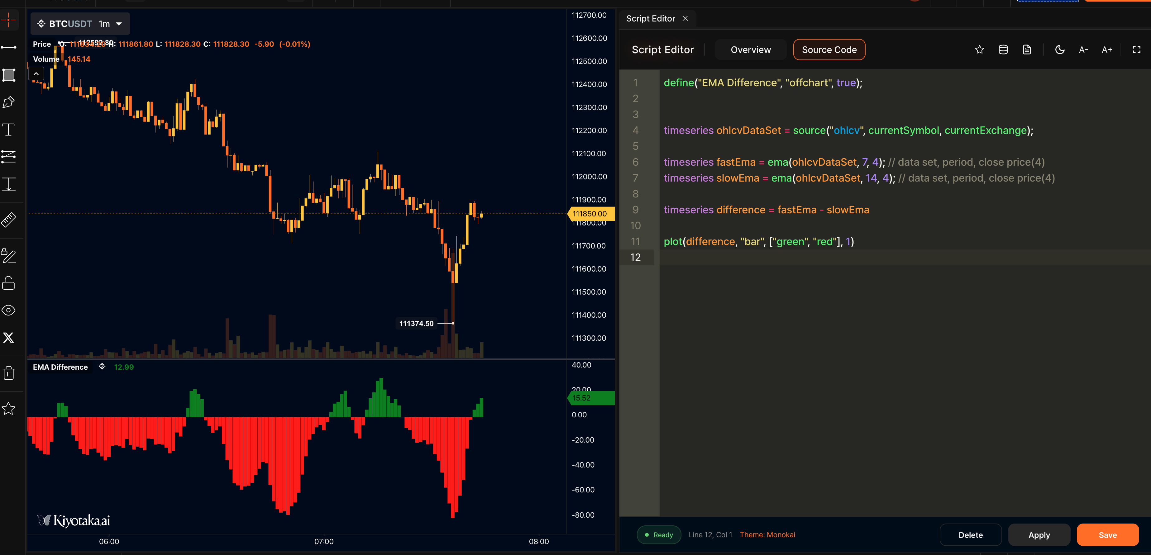
This guide walks you through creating your very first indicator in kScript. We'll build an off-chart indicator that plots the difference between two EMAs as bars.
Anatomy of a kScript
Every kScript has three main parts:
Definition
Define the name, title, and placement of your indicator.
Logic
Logic part of the script where you calculate the data that will be plotted.
Plot
Visualize the data.
Basic Script Structure
We'll build an off-chart indicator that plots the difference between two EMAs as bars. Every kScript v2 starts with a compiler annotation //@version=2 followed by a define() function that tells the platform what your script does and where to display it.
Explanation:
- //@version=2 - Required compiler annotation that tells kScript to use version 2 syntax and features
- "EMA Difference" - The display name in the UI
- "offchart" - Shows the indicator in a separate panel below the main chart
- true - Creates an independent Y-axis for better scaling
- "($fastPeriod, $slowPeriod)" - Adds input values to the title, so it displays as "EMA Difference (7, 14)"
Get the Data
To plot anything, we first need data. In kScript, that starts with subscribing to a data source. The ohlcv() function gives us OHLCV (trade data). For this example, we'll focus on close prices.
Data source explained:
- timeseries - A special type for time-series data. All other types can be declared using var
- ohlcv(...) - Gets OHLCV data of the current chart
- currentSymbol - Uses the currently selected trading pair
- currentExchange - Uses the currently selected exchange
💡 Pro Tip
Curious about the shape of this dataset? Click Apply, save the script, then hit the Data icon at the top to inspect it.
Build the Logic
Now let's calculate our EMAs. The standard library includes an ema() function. We'll calculate a fast EMA (7 periods) and slow EMA (14 periods), then find their difference.
EMA calculations:
- ema(ohlcvDataSet, 7, 4) - Fast EMA with 7 periods using close price (column 4)
- ema(ohlcvDataSet, 14, 4) - Slow EMA with 14 periods using close price (column 4)
- fastEma - slowEma - Calculate the difference between the two EMAs
💡 Pro Tip
You can inspect the difference dataset to confirm calculations by using the Data inspection feature.
Plot the Data
Now let's plot the difference as bars using the plotBar() function. We'll use green bars for positive values and red bars for negative values.
plotBar parameters:
- difference - The EMA difference data series to plot as bars
- ["green", "red"] - Color array for positive/negative bars
- colorIndex - Index to select specific color from colors array (0 for green, 1 for red)
- 1 - Bar width
Add User Inputs
Hardcoding values isn't very flexible. Instead, let's allow users to set the periods via inputs using the input() function. This makes your indicator customizable.
Input parameters:
- fastPeriod - Key for the input (used in code)
- "number" - Input type (number)
- 7 - Default value
- "Fast Period" - Label shown to users
Note: We use var instead of timeseries because user inputs are scalar values, not time series.
💡 Pro Tip
If you want to include the user settings in the indicator title, you can change the definition like this: define("EMA Difference", "offchart", true, "($fastPeriod, $slowPeriod)"); The title will then read as "EMA Difference (7, 14)".
Final Script
Here's your complete EMA Difference indicator script:
🎉 Congratulations!
You've built your first kScript indicator. Try experimenting with different functions, plots, and inputs next—the sky's the limit.